1. MNIST multiclass classifier with AML

This tutorial illustrates the use of AML by following a real example from preprocessing the dataset to performing inference. We have chosen to use the MNIST dataset for handwritten digits. In this tutorial we focus on multiclass classification of all 10 digits from 0 to 9. The dataset is used as is, and we do not introduce any prior knowledge (image augmetation, convolutional neural networks, etc).

You can request this tutorial as a Jupyter notebook and the AML libraries in Get access to AML Toolkit.

1.1. Load AML libraries

Most functionality to work with AML can be found in the root module:

import aml

1.2. Load MNIST dataset

The original dataset files:

• t10k-images-idx3-ubyte

• t10k-labels-idx1-ubyte

• train-images-idx3-ubyte

• train-labels-idx1-ubyte

The dataset can be downloaded from Yann Lecun MNIST database or Huggingface.

We provide a Python module, MNIST.py, with a series of helper functions to load and preprocess the dataset. The mnistGenerator searches and loads the datasets and provides functionality to load individual digits. The enum datasetType is used to select from which dataset (training, test or validation) samples come from.

from MNIST import mnistGenerator
from MNIST import datasetType

1.3. Embedding constants

A simple embedding for black and white images:

• constants for each black pixel B(i,j) (height x width),

• constants for each white pixel W(i,j) (height x width),

• constants for each label (10 if using all digits).

For instance, with 2x2 images the embedding set would be [B(1,1), B(1,2), B(2,1), B(2,2), W(1,1), W(1,2), W(2,1), W(2,2), label(1), label(2), ...]

1.3.1. Embedding function

We can use the following function to embed MNIST images.

An image is defined by a set of constants, one per pixel. Each constant will describe that pixel as white or black. For instance: [W(1,1), W(1,2), B(1,3), B(1,4), W(1,5), ... W(28,27), B(28,28)]

def digitToConstants(d):
    ss = MNIST_SIZE * MNIST_SIZE
    ret = [-1] * ss
    for j in range(ss):
        if d[j] > GRAY_THRESHOLD:
            ret[j] = j
        else:
            ret[j] = j + ss
    result = set(ret)
    return result

Images in the MNIST dataset have a size of 28x28 pixels. The constant MNIST_SIZE=28 holds the length of an image, and ss is a shorthand for the total number of pixels in an image. To embed these images, we need 2 times the total number of pixels in an image: 28x28 black pixels and 28x28 white pixels. The function digitToConstants creates a set that contains the indices for all the black pixels in the image (from 0 to ss), and the indices for all white pixels in the image (from ss to 2ss). Since the original images are grayscale, here we use a threshold to discriminate black and white pixels.

Notice that for this particular embedding, every pixel has to be either black (index j) or white (index j + ss), for a total of ss pixels. Here all terms, have the same number of embedding constants. This is due to the black and white constants being complementary. In other problems, different terms could have a different amount of embedding constants.

1.3.2. Functions to read examples and embed them as constants

These functions load images and embed them.

• mnistGenerator loads and preprocess the MNIST dataset. It can be queried to obtain images. The function takes one parameter indicating the size of the validation dataset. (It is common practice to have a validation dataset of 10000 elements.)

• getNextDigit returns an image and its label from one of the 3 datasets (training, test, and validation).

Finally, the image is expressed as embedding constants using digitToConstants and this set of constants is transformed into an AML term using LCSegment.

DATA_SOURCE = mnistGenerator(params.validationSize)
digit, label, _ = DATA_SOURCE.getNextDigit(typeOfDataset=typeOfDataset)
term = aml.LCSegment(digitToConstants(digit))

1.4. Training

1.4.1. Training parameters

First, we describe the parameters for training the model. Notice that AML uses hardly any hyperparameter, essentially only the mini batch size (initialPTrainingExamples and initialNTrainingExamples).

# Training iterations
iterations = 5000  # Maximum number of mini-batch iterations
num_batches_for_periodic_test = 10  # Report FPR and FPN on the test set
ranseed = 123456789

mnist_image_size = 28 * 28  # Number of pixels per image
mnist_numclasses = 10       # multi-class classifier
gray_threshold = 256 / 10

saveAtomization = False  # Save the model everytime a full test is performed

class trainingParameters:
    def __init__(self):
        self.constants = set()
        # Balance: number of times that false positives are overvalued over false negatives
        params.balance = mnist_numclasses - 1
        self.initialPTrainingExamples = 500
        self.initialNTrainingExamples = 500
        self.maxPTrainingExamples: int  # defined based on the dataset size
        self.maxNTrainingExamples: int  # defined based on the dataset size
        self.sizeOfFullTest: int        # defined based on the dataset size
        self.validationSize = 10000
        self.fullDatasetAtBatch = 500

1.4.2. Model and batch trainer initialisation

Initialise the model object that contains:

• the atomization, which is the model itself,

• the cmanager or constant manager, which contains information describing the constants (indices, names, etc).

model = sc.model()

Add to the constant manager in our model the embedding constants.

Notice that we also add a series of D constants representing each class (digit 0, digit 1, etc).

for i in params.constants:
    c = model.cmanager.setNewConstantIndex()

dTerm = [None] * mnist_numclasses
for i in range(0, mnist_numclasses):
    dIndex = cmanager.setNewConstantIndexWithName(f"D[{i}]")
    dTerm[i] = aml.LCSegment([dIndex])

When training, we also need to instantiate an embedder object that will take charge of all the details of training for one iteration (pinning terms, traces, dual model, etc). Check the Algebraic Machine Learning paper for a detailed explanation (https://arxiv.org/abs/1803.05252).

# Initialize the embedder for batch training
embedder = aml.sparse_crossing_embedder(model)
# If a positive duple produced new atoms during crossing, the duple is stored and reused in the following batch
embedder.params.storePositives = True
# The amount of atoms in the dual is reduced while keeping trace invariance
embedder.params.useReduceIndicators = True
# If enforceTraceConstraints is False a fresh atom is added to each constant every cycle.
embedder.params.enforceTraceConstraints = True
# Faster crossing only valid for binary classification
embedder.params.byQuotient = False
# True if the set of embedding constants does not change during training
embedder.params.staticConstants = True
# negativeIndicatorThreshold requires a minimal fraction of atoms from
#   negative Duples in the dual. The effect is to increase atom diversity.
embedder.params.negativeIndicatorThreshold = 0.1

1.4.3. Training loop

The training loop is simple. First we compute the new batch size. As the model matures, it processes relations faster, so it is usually a good idea to start with small batches and slowly grow over time. Having the batch size, we select a subset of relations. A relation is a tuple (image, label, positive/negative), to indicate whether certain image is a certain digit/label or not. Finally, we enforce those relations into the model.

# Start training
for batch in range(iterations):
    # Heuristics for computing minibatch size
    pBatchSize = min(
        ipBatchSize
        + batch * (fpBatchSize - ipBatchSize) / params.fullDatasetAtBatch,
        2 * fpBatchSize,
    )
    nBatchSize = min(
        inBatchSize
        + batch * (fnBatchSize - inBatchSize) / params.fullDatasetAtBatch,
        int(0.75 * fnBatchSize),
    )

    # Select minibatch
    tr_iterator, pbatch, nbatch = selectFromSet(
        trainingSet,
        tr_iterator,
        pBatchSize,
        nBatchSize,
    )

    # Enforce relation in the model
    embedder.enforce(pbatch, nbatch)

Below you can see the output of iteration 22.

... previous iterations ...

Selecting set
Updating unionModel... 7723
final unionModel size: 6677
 + region  1 > 416
 + region  2 > 394
 + region  3 > 460
 + region  4 > 484
 + region  5 > 416
 + region  6 > 427
 + region  7 > 382
 + region  8 > 465
 + region  9 > 516
 + region  10 > 489
 - region  1 > 2416
 - region  2 > 2369
 - region  3 > 2413
 - region  4 > 2404
 - region  5 > 2435
 - region  6 > 2439
 - region  7 > 2443
 - region  8 > 2379
 - region  9 > 2398
 - region  10 > 2406
Number of indicators 9355
Number of unique indicators 9355
Number of indicators 9355
Number of unique indicators 9355
Preparing space class
Calculating free traces
Number of indicators after selecting useful 7513
100% - Number of unique indicators after reduction 1978
Number of unique indicators after reduction 1696
Number of unique indicators after reduction 1597
Number of unique indicators after reduction 1592
Number of unique indicators after reduction 1592
Final number of indicators: 1592
Negative duple indicators 729
Calculating traces
From 36 to 36
Traces enforced with 36 atoms
From 3176 to 3176
Traces of constants
<Trace simplification> Result: 4648 to 2143
0% - (2143 ->  818) <Trace simplification> Result: 2687 to 2035
0% - (2035 ->  711) <Trace simplification> Result: 2468 to 2013
0% - (2013 ->  691) <Trace simplification> Result: 2539 to 2107

... more trace simplifications ...

92% - (3012 ->  1710) <Trace simplification> Result: 3880 to 3015
95% - (3015 ->  1713) <Trace simplification> Result: 3872 to 3037
97% - (3037 ->  1735) <Trace simplification> Result: 3914 to 3073
99% - (3073 ->  1772) <Trace simplification> Result: 3322 to 3034
CrossAll time: 6.249s
From 9711 to 7900
Stored 1813
L spectrum:
  L 1 atoms 1301
  L 2 atoms 10
  L 3 atoms 50
  L 4 atoms 115
  L 5 atoms 190
  L 6 atoms 237
  L 7 atoms 208
  L 8 atoms 177
  L 9 atoms 159
  L 10 atoms 150
  L 11 atoms 122
  L 12 atoms 70
  L 13 atoms 65
  L 14 atoms 47
  L 15 atoms 42
  L 16 atoms 21
  L 17 atoms 20
  L 18 atoms 14
  L 19 atoms 7
  L 20 atoms 8
  L 21 atoms 6
  L 22 atoms 3
  L 23 atoms 5
  L 24 atoms 3
  L 26 atoms 1
  L 28 atoms 1
  L 34 atoms 1
  L 35 atoms 1
Fraction of negative indicators: 0.45791457286432163, Union model fraction: 0
BATCH: 22 batchSize(2678, 24102) Classification error: 0.1556 UnionModel: 7900 (6410)


... following iterations ...

1.5. Postprocessing

Here you can explore the atomization in the last model: model.atomization.

But also the cumulative model that has been built combining the atomizations across the whole training process: embedder.unionModel.

print(f"{cGreen}Union model size:{cReset} {len(embedder.unionModel)}")
print(f"{cGreen}Size spectrum:{cReset}")
aml.printLSpectrum(embedder.unionModel)

print(f"{cGreen}Some random atoms:{cReset}")
import random
for at in random.choices(model.atomization, k=10):
    print(at.ucs)

embeddere.unionModel.sort(reverse=True,key=lambda at: len(at.ucs))
print(f"{cGreen}Largest atom{cReset}")
print(batchLearner.unionModel[0].ucs)

This shows information about the size of the model, for instance we expect both the union model and the atomization to grow rapidly in the initial phases of training and then plateau as we reach convergence. We can also display the size spectrum, that reports the number of atoms for each size. Initially, atoms are small and grow/mature with the number of batches. On the other hand, when the model finds patterns and is able to generalise, atoms tend to stabilise around an intermediate size. Very large atoms are generally caused by special cases, outliers or mislabels.

The above code block displays the following information for iteration 922:

Union model size: 10409
Size spectrum:
L spectrum:
  L 1 atoms 1496
  L 2 atoms 27
  L 3 atoms 193
  L 4 atoms 286
  L 5 atoms 509
  L 6 atoms 637
  L 7 atoms 755
  L 8 atoms 959
  L 9 atoms 992
  L 10 atoms 938
  L 11 atoms 852
  L 12 atoms 713
  L 13 atoms 572
  L 14 atoms 362
  L 15 atoms 254
  L 16 atoms 194
  L 17 atoms 167
  L 18 atoms 110
  L 19 atoms 75
  L 20 atoms 50
  L 21 atoms 54
  L 22 atoms 29
  L 23 atoms 33
  L 24 atoms 24
  L 25 atoms 18
  L 26 atoms 23
  L 27 atoms 13
  L 28 atoms 13
  L 29 atoms 7
  L 30 atoms 7
  L 31 atoms 6
  L 32 atoms 6
  L 33 atoms 8
  L 34 atoms 6
  L 35 atoms 1
  L 36 atoms 4
  L 37 atoms 5
  L 38 atoms 1
  L 39 atoms 2
  L 40 atoms 3
  L 41 atoms 2
  L 42 atoms 1
  L 44 atoms 2
Some random atoms:
bitarray({264})
bitarray({1184, 1568, 1351, 1512, 329, 303, 1136, 595, 596, 215, 125, 574})
bitarray({222})
bitarray({320, 1217, 1568, 357, 1134, 496, 1425, 1330, 244, 1268, 1052})
bitarray({1568, 129, 1220, 1535, 1165, 1293, 271, 592, 597, 1304, 217, 1437, 351})
bitarray({992, 513, 1568, 1029, 1194, 491, 939, 397, 653, 655, 1100, 690, 243, 1235, 1364, 1078, 539, 157})
bitarray({582})
bitarray({164})
bitarray({1568, 1134, 1044, 398})
bitarray({746})
Largest atom
bitarray({1280, 1408, 1160, 1162, 651, 1168, 657, 659, 1050, 1568, 289, 162, 425, 554, 1193, 1323, 302, 1198, 321, 970, 1357, 206, 1102, 208, 593, 1107, 1108, 215, 1113, 218, 348, 483, 996, 1251, 359, 1386, 620, 1132, 1133, 1136, 1137, 1267, 244, 509})

1.5.1. Plotting results

For classification problems with square images the viewer module provides some functions to plot atoms. It simply maps back constant indices to their position and color on an image. It then uses matplotlib to output the results.

import viewer as av

theViewer = av.atomViewer_bw_sq_image(
    cmanager=model.cmanager,
    min_size=2,
    scale=10,
    atoms_per_board=[10, 10],
)
theViewer.save(f"RESULTS/MNIST_IMG_{targetDigit}_{i}", batchLearner.unionModel)
theViewer.save(f"RESULTS/MNIST_IMG_model_{targetDigit}_{i}", model.atomization)

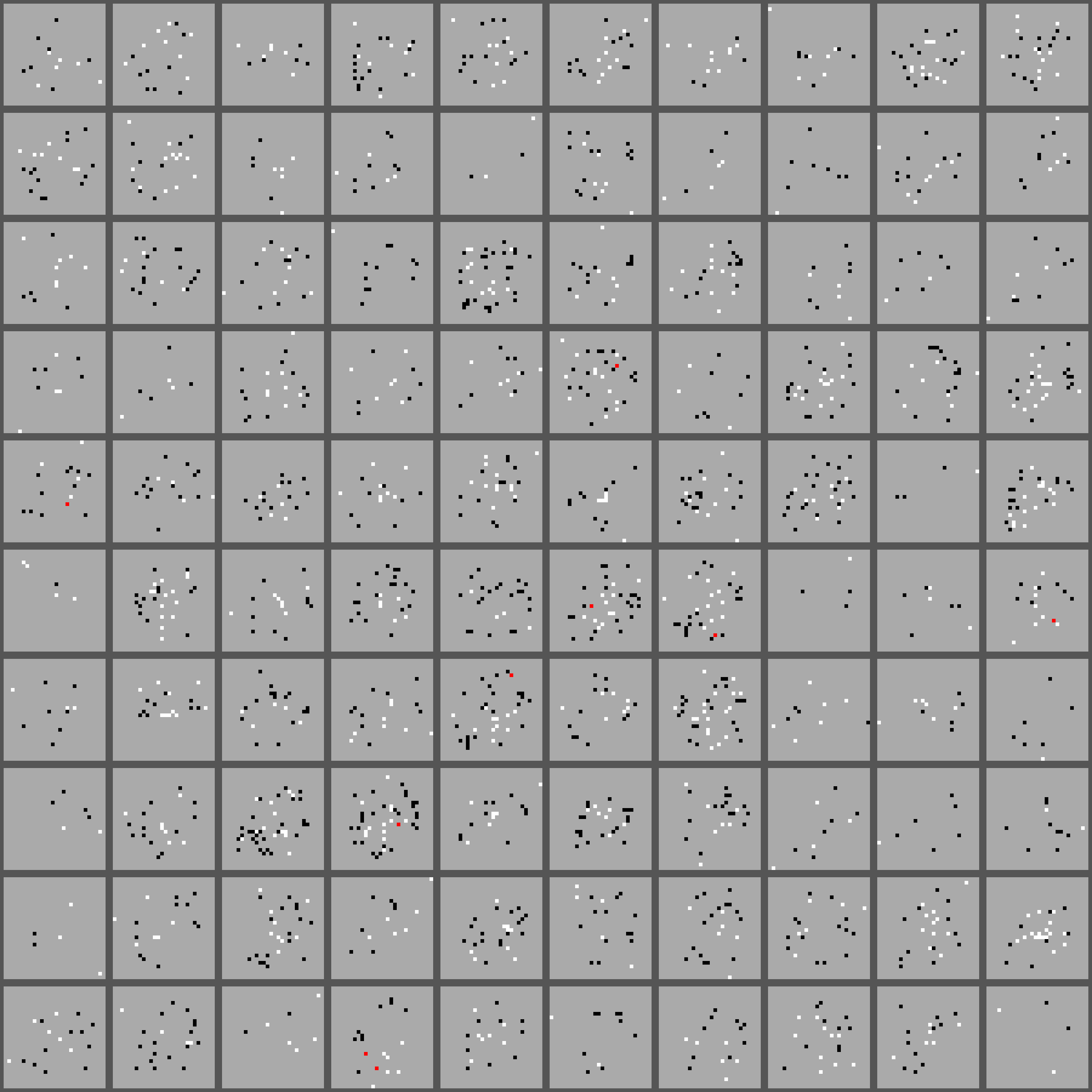
As an example, below we show 100 atoms in model.atomization. Black and white pixels indicate that the constant is present in the atom; red, that both constants are present; and gray, that none is present.

1.5.2. Inference

To perform inference in AML we first build a duple, and then we ask the model whether that duple is positive or not. This is done by checking the atoms from its terms. When a duple \(T_L < T_R\) is in the model then all atoms in \(T_L\) are also part of \(T_R\). In that case we say that there are no missing atoms, or no misses. If on the other hand, many atoms are missing, then the duple is not present in the model.

The following function computes the atoms that are present in \(T_L\) but are missing in \(T_R\) of a duple.

def computeMisses(leftTerm, rightTerm, atomization):
    atomsInLeftTerm = aml.atomsIn(atomization, leftTerm)
    atomsMissingInRight = aml.atomsNotIn(atomsInLeftTerm, rightTerm)
    return atomsMissingInRight

Finally, using the above functions we can compute the number of missing atoms from a set of positive and negative examples.

def mnistDigitTest(targetDigit):
    d, _, _ = DATA_SOURCE.getNextDigit(targetDigit, False, datasetType.test)
    result = digitToConstants(d)
    return aml.LCSegment(result)
def mnistOtherDigitTest(targetDigit):
    d, _, _ = DATA_SOURCE.getNextDigit(targetDigit, True, datasetType.test)
    result = digitToConstants(d)
    return aml.LCSegment(result)

positiveExampleTerm = [mnistDigitTest(targetDigit) for _ in range(10)]
negativeExampleTerm = [mnistOtherDigitTest(targetDigit) for _ in range(10)]

missesPositiveExamples = [computeMisses(dTerm[targetDigit], ex, embedder.unionModel) for ex in positiveExampleTerm]
missesNegativeExamples = [computeMisses(dTerm[targetDigit], ex, embedder.unionModel) for ex in negativeExampleTerm]

print("Positive Class:")
print([len(misses) for misses in missesPositiveExamples])
print("Negative Class:")
print([len(misses) for misses in missesNegativeExamples])

The result for a random subset of samples:

Positive Class:
[0, 0, 0, 0, 4, 2, 0, 0, 0, 0]
Negative Class:
[26, 9, 16, 18, 10, 15, 13, 15, 8, 24]

For the positive class we are taking images with the same label as the target digit, therefore we expect the model to show very few misses. As we see, some images had a few misses, but most cases the match was perfect.

For the negative class we choose at random images different to the target digit, we then expect the model to show many misses, indicating that the label and the images are not related. Here we see a high number of misses. The lowest number of misses is twice as large as the maximum error for the positive class.